mod <- lm(mpg ~ wt, data = mtcars)
summary(mod)
#>
#> Call:
#> lm(formula = mpg ~ wt, data = mtcars)
#>
#> Residuals:
#>     Min      1Q  Median      3Q     Max
#> -4.5432 -2.3647 -0.1252  1.4096  6.8727
#>
#> Coefficients:
#>             Estimate Std. Error t value Pr(>|t|)
#> (Intercept)  37.2851     1.8776  19.858  < 2e-16 ***
#> wt           -5.3445     0.5591  -9.559 1.29e-10 ***
#> ---
#> Signif. codes:  0 '***' 0.001 '**' 0.01 '*' 0.05 '.' 0.1 ' ' 1
#>
#> Residual standard error: 3.046 on 30 degrees of freedom
#> Multiple R-squared:  0.7528, Adjusted R-squared:  0.7446
#> F-statistic: 91.38 on 1 and 30 DF, p-value: 1.294e-10Side-effect soup
Side-effect soup occurs when you mix side-effects and regular computation within the same function.
What is a side-effect?
There are two main types of side-effect:
- those that give feedback to the user.
- those that change some global state.
User feedback
Global state
Creating (or modifying) an existing binding with
<-.Modifying the search path by attaching a package with
library().Changing the working directory with
setwd().Modifying a file on disk with (e.g.)
write.csv().Changing a global option with
options()or a base graphics parameter withgpar().Setting the random seed with
set.seed()Installing a package.
Changing environment variables with
Sys.setenv(), or indirectly via a function likeSys.setlocale().Modifying a variable in an enclosing environment with
assign()or<<-.Modifying an object with reference semantics (like R6 or data.table).
More esoteric side-effects include:
Detaching a package from the search path with
detach().Changing the library path, where R looks for packages, with
.libPaths()Changing the active graphics device with (e.g.)
png()ordev.off().Registering an S4 class, method, or generic with
methods::setGeneric().Modifying the internal
.Random.seed
What are some examples?
-
The summary of a linear model includes a p-value for the overall
regression. This value is only computed when the summary is printed: you can see it but you can’t touch it.
Why is it bad?
Side-effect soup is bad because:
If a function does some computation and has side-effects, it can be challenging to extract the results of computation.
-
Makes code harder to analyse because it may have non-local effects. Take this code:
x <- 1
y <- compute(x)
z <- calculate(x, y)

df <- data.frame(x = "x")
If
compute()orcalculate()don’t have side-effects then you can predict whatdfwill be. But ifcompute()didoptions(stringsAsFactors = FALSE)thendfwould now contain a character vector rather than a factor.
Side-effect soup increases the cognitive load of a function so should be used deliberately, and you should be especially cautious when combining them with other techniques that increase cognitive load like tidy-evaluation and type-instability.
How avoid it?
Localise side-effects
Constrain the side-effects to as small a scope as possible, and clean up automatically to avoid side-effects. withr
Extract side-effects
It’s not side-effects that are bad, so much as mixing them with non-side-effect code.
Put them in a function that is specifically focussed on the side-effect.
If your function is called primarily for its side-effects, it should return the primary data structure (which should be first argument), invisibly. This allows you to call it mid-pipe for its side-effects while allow the primary data to continue flowing through the pipe.
Make side-effects noisy
Primary purpose of the entire package is side-effects: modifying files on disk to support package and project development. usethis functions are also designed to be noisy: as well as doing it’s job, each usethis function tells you what it’s doing.
But some usethis functions are building blocks for other more complex tasks.
Provide an argument to suppress
You’ve probably used base::hist() for it’s side-effect of drawing a histogram:
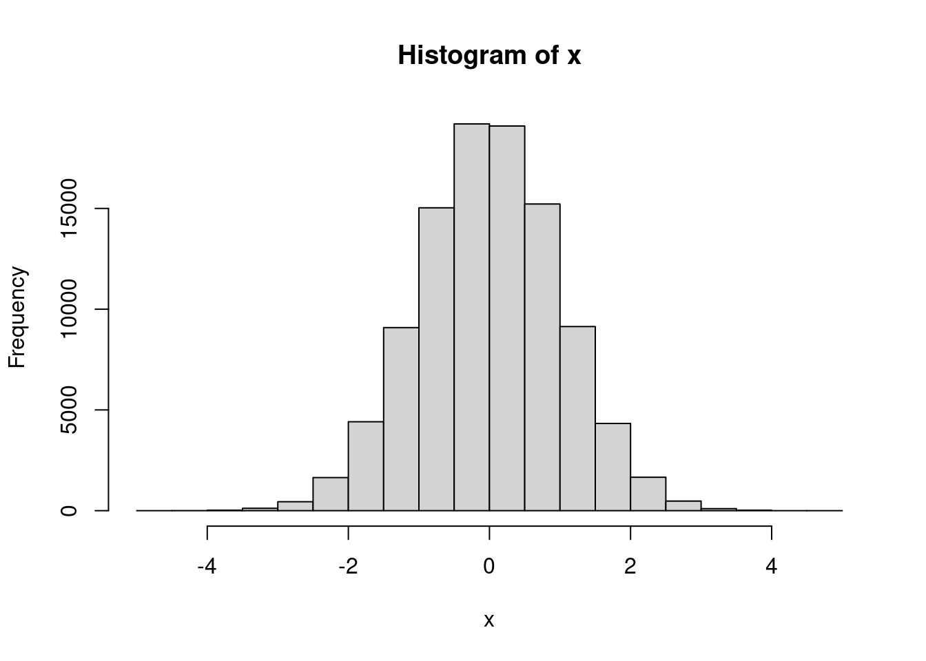
But you might not know that hist() also returns the result of the computation. If you call plot = FALSE it will simply return the results of the computation:
xhist <- hist(x, plot = FALSE)
str(xhist)
#> List of 6
#>  $ breaks  : num [1:21] -5 -4.5 -4 -3.5 -3 -2.5 -2 -1.5 -1 -0.5 ...
#>  $ counts  : int [1:20] 1 2 23 120 444 1643 4414 9086 15031 19196 ...
#>  $ density : num [1:20] 0.00002 0.00004 0.00046 0.0024 0.00888 ...
#>  $ mids    : num [1:20] -4.75 -4.25 -3.75 -3.25 -2.75 -2.25 -1.75 -1.25 -0.75 -0.25 ...
#>  $ xname   : chr "x"
#>  $ equidist: logi TRUE
#>  - attr(*, "class")= chr "histogram"
This is a good approach for retro-fitting older functions while making minimal API changes. However, I think it dilutes a function to be both used for plotting and for computing so should be best avoided in newer code.
Use the print() method
An alternative approach would be to always return the computation, and instead perform the output in the print() method.
Of course ggplot2 isn’t perfect: it creates an object that specifies the plot, but there’s no easy way to extract the underlying computation so if you’ve used geom_smooth() to add lines of best fit, there’s no way to extract the values. Again, you can see the results, but you can’t touch them, which is very frustrating!
Make easy to undo
If all of the above techniques fail, you should at least make the side-effect easy to undo. A use technique to do this is to make sure that the function returns the previous values, and that it can take it’s own input.
This is how options() and par() work. You obviously can’t eliminate those functions because their complete purpose is have global changes! But they are designed in such away that you can easily undo their operation, making it possible to apply on a local basis.
There are two key ideas that make these functions easy to undo:
-
They invisibly return the previous values as a list:
-
Instead of
nnamed arguments, they can take a single named list:(I wouldn’t recommend copying this technique, but I’d instead recommend always taking a single named list. This makes the function because it has a single way to call it and makes it easy to extend the API in the future, as discussed in Chapter 23)
Together, this means that you easily can set options temporarily.:
If temporarily setting options in a function, you should always restore the previous values using on.exit(): this ensures that the code is run regardless of how the function exits.
Package considerations
Code in package is executed at build-time.i.e. if you have:
x <- Sys.time()For mac and windows, this will record when CRAN built the binary. For linux, when the package was installed.
Beware copying functions from other packages:
foofy <- barfy::foofyVersion of barfy might be different between run-time and build-time.
Introduces a build-time dependency.